Understanding SFT from an RL Perspective

Introduction

SFT and RL are both common post-training techniques. Interestingly, they are deeply related: from the gradient perspective, SFT is performing a special kind of policy gradient; from the loss perspective, the SFT loss is a lower bound of the RL loss.

In this post, I will walk through the mathematical connection between SFT and RL, along with three SFT improvement algorithms inspired by this connection: DFT, PSFT, and ASFT.

Basic Formulas of SFT and RL

First, let us set up the notation: x is the prompt, y is the model's own output, y* is the expert output, the model being fine-tuned is π_θ, and the RL reward function is r(x, y).

SFT aims to fit the expert output distribution given a prompt:

$$\mathcal{L}_{\mathrm{SFT}}(\theta) = \mathbb{E}_{(x,\, y^*) \sim \mathcal{D}} \big[ -\log \pi_\theta(y^* \mid x) \big].$$

Its gradient is:

$$\nabla_\theta \mathcal{L}_{\mathrm{SFT}}(\theta) = \mathbb{E}_{(x,\, y^*) \sim \mathcal{D}} \big[ -\nabla_\theta \log \pi_\theta(y^* \mid x) \big].$$

RL aims to improve the policy's reward:

$$J(\theta) = \mathbb{E}_{x \sim \mathcal{D}_x,\; y \sim \pi_\theta(\cdot \mid x)} \big[ r(x, y) \big].$$

The sentence-level policy gradient is:

$$\nabla_\theta J(\theta) = \mathbb{E}_{x \sim \mathcal{D}_x,\; y \sim \pi_\theta(\cdot \mid x)} \big[ \nabla_\theta \log \pi_\theta(y \mid x) \, r(x, y) \big].$$

It is generally believed that SFT is simple and fast, but has a limited performance ceiling (its biggest weakness is insufficient generalization [4]); RL is the opposite. In the post-training of large language models, SFT typically serves as a precursor to RL, providing a more stable starting point.

SFT Is Performing Sparse On-Policy RL

The training samples in SFT generally come from a stronger model or from humans (rather than from the model itself), so the optimization process is off-policy.

Through resampling and reweighting, the SFT objective can be rewritten in an on-policy form:

$$\mathbb{E}_{(x,\, y^*) \sim \mathcal{D}} \big[ -\nabla_\theta \log \pi_\theta(y^* \mid x) \big] = \mathbb{E}_{x \sim \mathcal{D}_x} \; \underbrace{\mathbb{E}_{y \sim \pi_\theta(\cdot \mid x)} \left[ \frac{\mathbf{1}[y = y^*]}{\pi_\theta(y \mid x)} \big[ -\nabla_\theta \log \pi_\theta(y \mid x) \big] \right]}_{\text{resample + reweight}}$$

The intuition here is: in theory, there is a nonzero probability of sampling the expert output (even if that probability may be extremely low), so mathematically we can rewrite the formula via resampling; and to keep the expectation consistent, we must weight that lucky sample of the expert output inversely proportional to its sampling probability (the denominator part).

If we define:

$$w(y \mid x) = \frac{1}{\pi_\theta(y \mid x)}, \qquad r(x, y) = \mathbf{1}[\, y = y^* \,].$$

where w(y|x) is the importance weight, and r(x, y) is the SFT reward function (reward = 1 if and only if y = y*).

Then the SFT gradient can be rewritten as:

$$\nabla_\theta \mathcal{L}_{\mathrm{SFT}}(\theta) = -\, \mathbb{E}_{x \sim \mathcal{D}_x,\; y \sim \pi_\theta(\cdot \mid x)} \big[ w(y \mid x) \, \nabla_\theta \log \pi_\theta(y \mid x) \, r(x, y) \big].$$

Recall that the RL policy gradient is:

$$\nabla_\theta J(\theta) = \mathbb{E}_{x \sim \mathcal{D}_x,\; y \sim \pi_\theta(\cdot \mid x)} \big[ \nabla_\theta \log \pi_\theta(y \mid x) \, r(x, y) \big].$$

So, mathematically, we can treat the SFT gradient update as an on-policy gradient process.

However, SFT has two special properties:

1. The SFT reward is very sparse. Reward = 1 if and only if y = y*; in all other cases, the reward is 0.
2. The SFT gradient distribution is high-variance. The gradient is inversely proportional to w(y|x): the harder a sample is to learn (i.e., the smaller π_θ(y|x) is), the larger the importance weight will be, and thus the larger the gradient — which brings training instability and overfitting.

DFT: Dynamically Down-weighting the Gradient

DFT was proposed to mitigate property 2. Its method is to multiply the token-level gradient by an inverse-probability factor that cancels out the importance weight, thereby down-weighting excessively large gradients.

The DFT loss is:

$$\mathcal{L}_{\mathrm{DFT}}(\theta) = \mathbb{E}_{(x,\, y^*) \sim \mathcal{D}} \left[ -\sum_{t=1}^{|y^*|} \operatorname{sg}\!\big( \pi_\theta(y^*_t \mid y^*_{<t}, x) \big) \, \log \pi_\theta(y^*_t \mid y^*_{<t}, x) \right].$$

where sg = stop gradient, i.e., this term does not participate in backpropagation.

Intuitively, DFT suppresses the model's tendency to "memorize the training data": tokens that are hard to learn are no longer forced upon the model. By curbing overfitting, improvements in generalization and overall performance become possible.

According to the original paper's experiments, DFT noticeably improves model performance on math reasoning data.

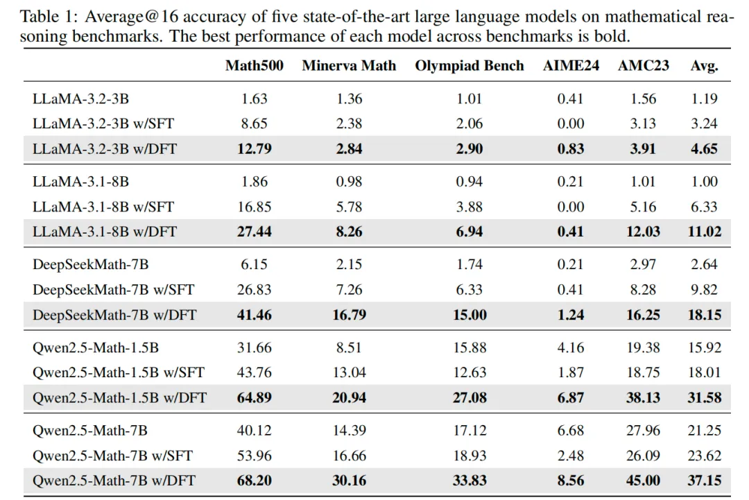
Later in this post, we will revisit DFT from another mathematical angle.

For the detailed mathematical derivations in this section, see the DFT paper.

PSFT: Borrowing from PPO

As mentioned above, SFT can be viewed as a policy gradient process, so a natural idea is: directly bring advanced RL algorithms (such as PPO) into SFT.

PSFT is exactly this idea.

Let us first look at the PPO objective:

$$L^{\mathrm{CLIP}}(\theta) = \hat{\mathbb{E}}_{(s_t,\, a_t) \sim \pi_{\theta_{\mathrm{old}}}} \left[ \min \big( r_t(\theta) \hat{A}_t, \; \operatorname{clip}\big( r_t(\theta),\, 1 - \epsilon,\, 1 + \epsilon \big) \hat{A}_t \big) \right].$$

The PSFT loss function directly borrows from PPO:

$$L^{\mathrm{PSFT}}(\theta) = \mathbb{E}_{(s_t,\, a_t) \sim \mathcal{D}} \left[ \min \left( \frac{\pi_\theta(a_t \mid s_t)}{\pi_{\theta_{\mathrm{old}}}(a_t \mid s_t)}, \; \operatorname{clip}\!\left( \frac{\pi_\theta(a_t \mid s_t)}{\pi_{\theta_{\mathrm{old}}}(a_t \mid s_t)},\, 1 - \epsilon,\, 1 + \epsilon \right) \right) \right].$$

Here, s_t corresponds to the prompt, a_t corresponds to the output token, π_θ_old corresponds to the pre-update policy (the base model, optionally after a warm-up), and π_θ is the model being optimized. Since the SFT reward is an identity function with value 1, the advantage A_t can be dropped, and sampling is done from the offline dataset D.

From the gradient perspective, the PSFT gradient update works as follows:

$$\begin{aligned} &\nabla_\theta L^{\mathrm{PSFT}}(\theta) = \mathbb{E}_{(s_t,\, a_t) \sim \mathcal{D}} \big[ r_t(\theta) \cdot \mathbb{I}_{\mathrm{trust}}(r_t(\theta)) \cdot \nabla_\theta \log \pi_\theta(a_t \mid s_t) \big], \\ &\text{where } \quad \mathbb{I}_{\mathrm{trust}}(r_t(\theta)) = \begin{cases} 0, & r_t(\theta) > 1 + \epsilon, \\ 1, & \text{otherwise.} \end{cases} \end{aligned}$$

where

$$r_t(\theta) = \frac{\pi_\theta(a_t \mid s_t)}{\pi_{\theta_{\mathrm{old}}}(a_t \mid s_t)}$$

is the importance ratio between the current policy π_θ and the pre-update policy π_θ_old.

Intuitively, the effect of PSFT is: for samples whose data distributions differ greatly, no gradient update is performed, thereby avoiding large policy updates. This idea is similar to DFT, except that DFT dynamically down-weights gradients, while PSFT truncates gradients within a trust region.

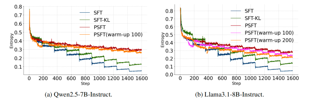
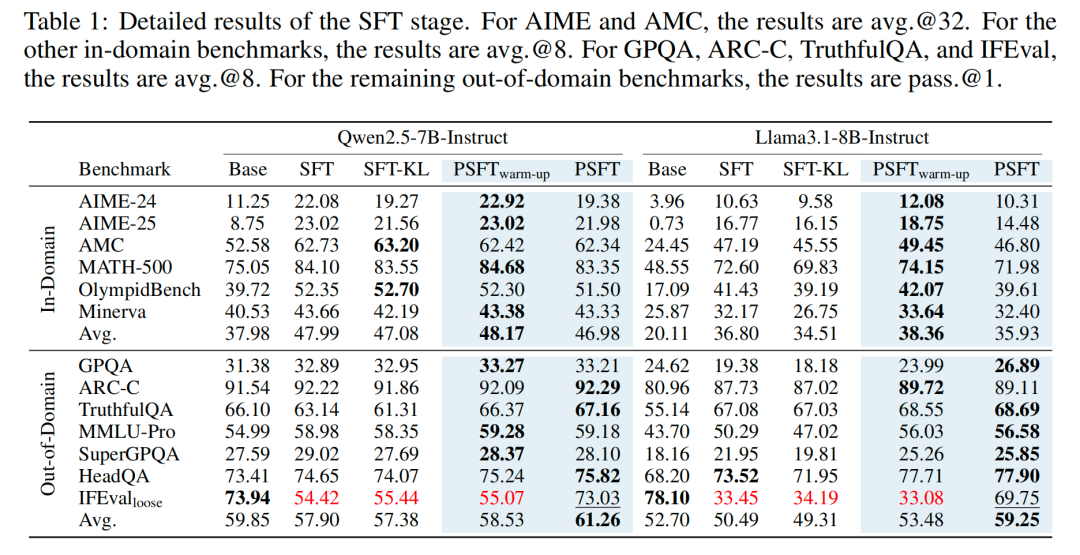
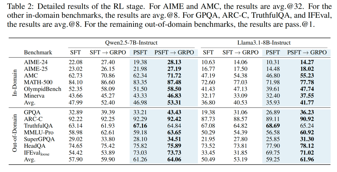
From the original paper's experiments, the properties of PSFT are:

• It prevents entropy collapse (which is very friendly for the subsequent RL stage);

• It better preserves out-of-domain capability, though in-domain capability drops somewhat; adding a warm-up (running a few SFT steps first) can bring higher in-domain accuracy, but at the cost of some out-of-domain performance;

• It works better as a starting point for RL.

SFT Is a Lower Bound of RL

In this section, let us revise the notation: let τ denote a model trajectory (the prompt together with the model's response), the model being fine-tuned be π_θ with parameters θ, the reference policy be π_ref, and the RL reward function be R.

Let us revisit the RL objective:

$$J(\theta) = \mathbb{E}_{\tau \sim \pi_\theta} \big[ R(\tau) \big]$$

Using the resample-and-reweight trick (similar to the previous section), it can be rewritten as an expectation under the reference policy π_ref:

$$J(\theta) = \mathbb{E}_{\tau \sim \pi_{\mathrm{ref}}} \left[ \frac{\pi_\theta(\tau)}{\pi_{\mathrm{ref}}(\tau)} R(\tau) \right]$$

The purpose of this step is to make the data sampling distribution consistent with SFT, so that the subsequent comparison with SFT becomes easier.

To more conveniently analyze the tightness of the lower bound, we introduce an auxiliary distribution q(τ) and rewrite the objective as:

$$J(\theta) = \mathbb{E}_{\tau \sim \pi_{\mathrm{ref}}} \left[ \frac{q(\tau)}{\pi_{\mathrm{ref}}(\tau)} \cdot \frac{\pi_\theta(\tau)}{q(\tau)} R(\tau) \right]$$

Applying the elementary inequality x ≥ 1 + log x (which follows from the concavity of the logarithm) to the ratio π_θ(τ)/q(τ), we get:

$$\frac{\pi_\theta(\tau)}{q(\tau)} \geq 1 + \log \frac{\pi_\theta(\tau)}{q(\tau)} = 1 + \log \pi_\theta(\tau) - \log q(\tau)$$

Substituting it back into the objective, we obtain:

$$\begin{aligned} J(\theta) &\geq \mathbb{E}_{\tau \sim \pi_{\mathrm{ref}}} \left[ \frac{q(\tau)}{\pi_{\mathrm{ref}}(\tau)} \big( 1 + \log \pi_\theta(\tau) - \log q(\tau) \big) R(\tau) \right] \\ &= \mathbb{E}_{\tau \sim \pi_{\mathrm{ref}}} \left[ \frac{q(\tau)}{\pi_{\mathrm{ref}}(\tau)} R(\tau) \right] + \mathbb{E}_{\tau \sim \pi_{\mathrm{ref}}} \left[ \frac{q(\tau)}{\pi_{\mathrm{ref}}(\tau)} R(\tau) \log \pi_\theta(\tau) \right] \\ &\quad - \mathbb{E}_{\tau \sim \pi_{\mathrm{ref}}} \left[ \frac{q(\tau)}{\pi_{\mathrm{ref}}(\tau)} R(\tau) \log q(\tau) \right] \end{aligned}$$

If q(τ) is independent of the model parameters θ (it can be controlled by humans), then the first and third terms can both be treated as a constant const; meanwhile, in the SFT context, since R is an identity function and reward = 1, we define a data distribution D+ used for SFT training, and the R part can be dropped. In summary, the inequality can be rewritten as:

$$J(\theta) \geq c_{\mathrm{ref}} \, \mathbb{E}_{\tau \in D^+} \left[ \frac{q(\tau)}{\pi_{\mathrm{ref}}(\tau)} \log \pi_\theta(\tau) \right] + \mathrm{const}$$

where $c_{\mathrm{ref}} = P_{\pi_{\mathrm{ref}}}(\tau \in D^+)$.

where D+ denotes the distribution of expert (demonstration) data.

Based on this inequality, we can conclude:

• Setting q(τ) = π_ref(τ), then after the fraction cancels out, the right-hand side of the inequality (excluding the constant part) is exactly the SFT loss; therefore, the SFT loss is a lower bound of the RL loss;
• When does this lower bound become tighter (i.e., closer to the RL loss)? Going back to the inequality x ≥ 1 + log x: the closer x is to 1, the tighter the bound; since $x = \frac{\pi_\theta(\tau)}{q(\tau)}$, the closer q is to π_θ, the closer this lower bound gets to the RL loss.

DFT Is a Tighter Lower Bound

Let us revisit DFT.

Substituting DFT into the formula derived at the end of the previous section and solving for its q, we get:

$$q(\tau) = \frac{\pi_{\mathrm{ref}}(\tau \mid D^+) \, \operatorname{sg}[p_\theta(\tau)]}{\mathbb{E}_{\tau \sim \pi_{\mathrm{ref}}(\cdot \mid D^+)} \big[ \operatorname{sg}[p_\theta(\tau)] \big]}$$

Note that because the stop-gradient operation is applied, q still remains independent of the model parameters during optimization, so the condition above is satisfied.

However, this formula is too complicated and not intuitive, but it can be mathematically simplified. Writing the q distribution at the k-th training iteration, we get:

$$q_k(\tau) \propto \pi_{\mathrm{ref}}(\tau \mid D^+) \, p_{\theta_k}(\tau)$$

Intuitively, since DFT's q distribution incorporates the model probability (as a constant, not participating in gradient computation), its distribution is closer to the model's own distribution. Combined with the second conclusion of the previous section, we get: compared with the SFT loss, the DFT loss is a tighter lower bound of the RL loss.

For the detailed mathematical derivations in this section, see the ASFT paper.

ASFT: Mitigating DFT's Collapse Problem

However, DFT carries the risk of model collapse.

Let us revisit DFT's q distribution:

$$q_k(\tau) \propto \pi_{\mathrm{ref}}(\tau \mid D^+) \, p_{\theta_k}(\tau)$$

There is a feedback loop here: samples with larger $p_\theta$ are more likely to be sampled → which makes their $p_\theta$ even larger → in the next iteration these samples are even more likely to be sampled → and so on in a loop, causing the training distribution to become increasingly peaked, until model collapse.

Forward KL is well suited to solving the model collapse problem [5], so ASFT adds forward KL to the DFT loss:

$$\mathcal{L}_{\mathrm{ASFT}}(\theta) = \mathcal{L}_{\mathrm{DFT}}(\theta) + \lambda \, \mathbb{E}_{s} \big[ D_{\mathrm{KL}}\big( \pi_{\mathrm{base}}(\cdot \mid s) \,\|\, \pi_\theta(\cdot \mid s) \big) \big]$$

As a result, ASFT is not only a tighter lower bound of the RL loss (like DFT), but also mitigates model collapse.

Let us pick the experiments from the ASFT paper to see how DFT and ASFT perform.

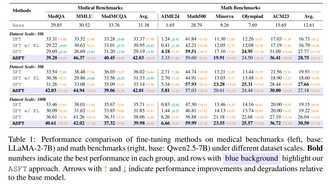
From the paper's experimental results, we can find:

1. On math reasoning tasks (the right half of the table), both DFT and ASFT outperform SFT;
2. On medical knowledge tasks, DFT may even underperform SFT, while ASFT beats both DFT and SFT;
3. Adding only the KL term does not make SFT better — on the contrary, it hinders its learning process.

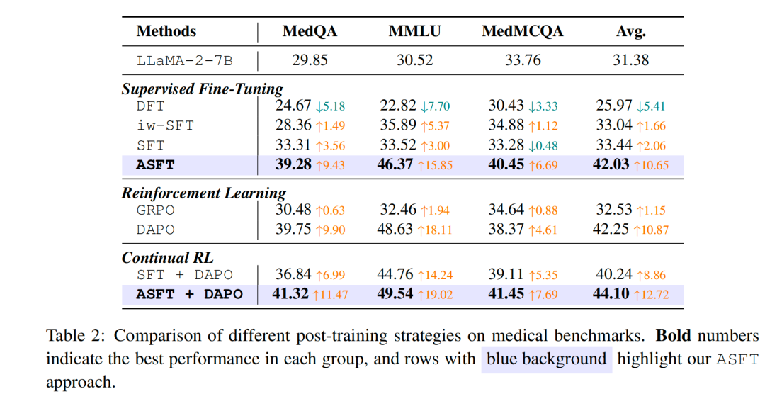
If RL training is performed after ASFT, the advantage brought by ASFT is also preserved.

Summary

This post draws a hidden line connecting SFT and RL — two techniques that seem worlds apart — from both the gradient and loss perspectives, which is illuminating for understanding the limitations of SFT.

We also introduced three improved SFT algorithms: DFT, PSFT, and ASFT. Readers are encouraged to try these methods on their own business scenarios. The ideas behind them are also worth borrowing — suppress SFT's overfitting tendency (avoid over-memorizing the training data), but do not fall into model collapse. That said, regarding solving the sparse reward problem, none of the algorithms covered in this post addresses it — yet it remains an equally promising optimization direction.

References

[1] ON THE GENERALIZATION OF SFT: A REINFORCEMENT LEARNING PERSPECTIVE WITH REWARD RECTIFICATION — arxiv.org/pdf/2508.05629

[2] PROXIMAL SUPERVISED FINE-TUNING — arxiv.org/pdf/2508.17784

[3] Anchored Supervised Fine-Tuning — arxiv.org/pdf/2509.23753

[4] SFT Memorizes, RL Generalizes: A Comparative Study of Foundation Model Post-training — arxiv.org/pdf/2501.17161

[5] The Difference Between Forward and Reverse KL — duanyu.github.io/kl