There Is No Single Best SFT Loss

Paper: Beyond Log Likelihood: Probability-Based Objectives for Supervised Fine-Tuning across the Model Capability Continuum (thanks to a reader on Xiaohongshu for recommending this one).

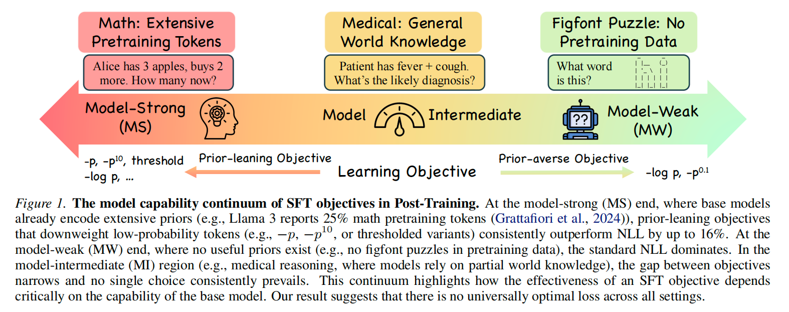
Figure 1: The model capability continuum of SFT objectives in post-training — prior-leaning objectives dominate at the model-strong end, NLL dominates at the model-weak end, and no single objective prevails in between

A Parametrized Family of SFT Objectives

First, the paper uses a parametrized family to abstract SFT objectives:

f(p) = -\, \frac{p^{\alpha} - 1}{\alpha}

When α = 0, this reduces to f(p) = −log p — the standard negative log-likelihood (NLL) loss.

Different values of α give different gradient structures:

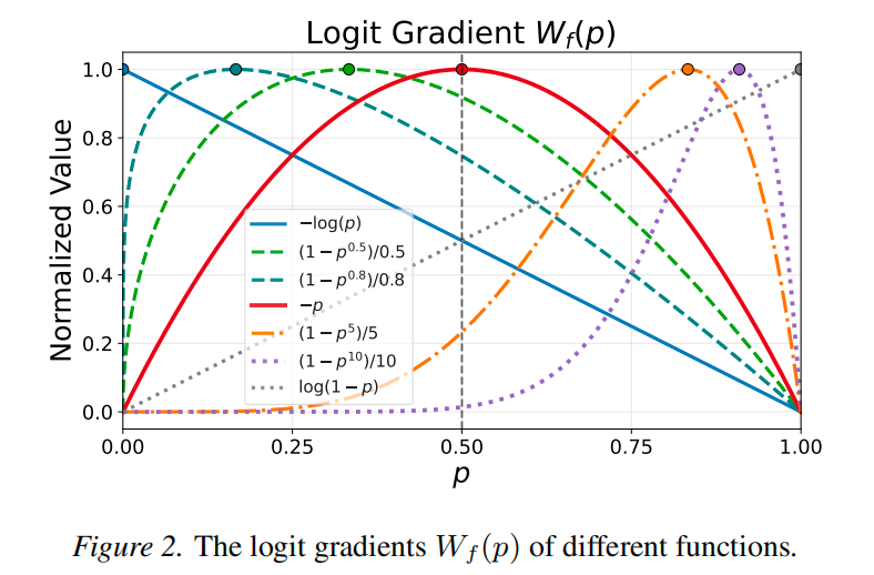
Figure 2: The logit gradients W_f(p) of different objective functions — the gradient peak shifts from low-probability to mid/high-probability tokens as α grows

When α is small, low-probability tokens receive larger gradients; when α is large, mid- and high-probability tokens receive larger gradients.

Prior-Leaning vs. Prior-Averse

The paper defines two classes of SFT strategies:

Prior-leaning: reinforces the model's existing (prior) abilities, assigning larger gradients to mid- and high-probability tokens;
Prior-averse: corrects the model's prior, assigning larger gradients to low-probability tokens.

Under this framing:

−log p (α = 0) is prior-averse;
−p (α = 1) is prior-leaning;
−log p + a threshold (i.e., not learning low-probability tokens at all) is also prior-leaning.

The Key Finding: It Depends on the Model's Prior

The paper studies the relationship between (prior-leaning vs. prior-averse; strength of the model's prior) and task performance. The conclusion:

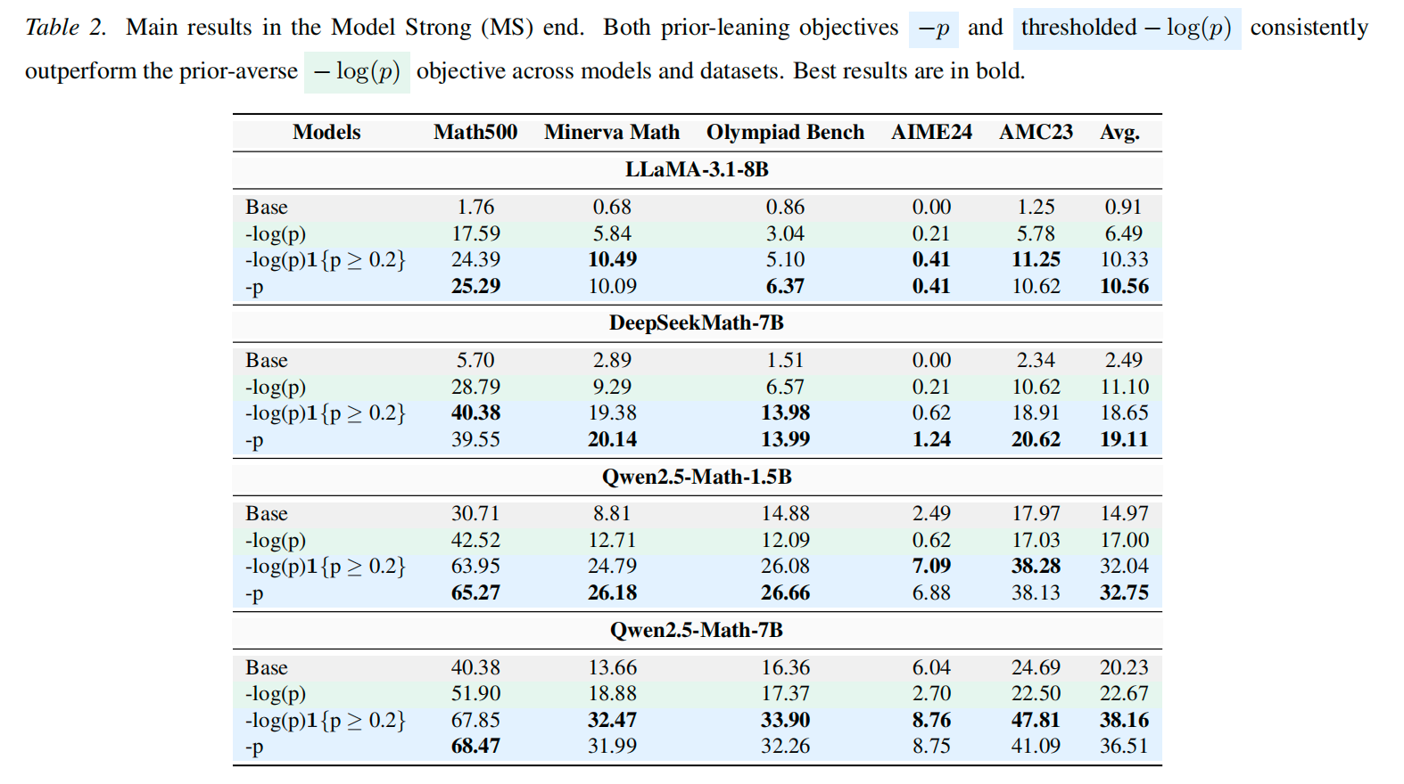
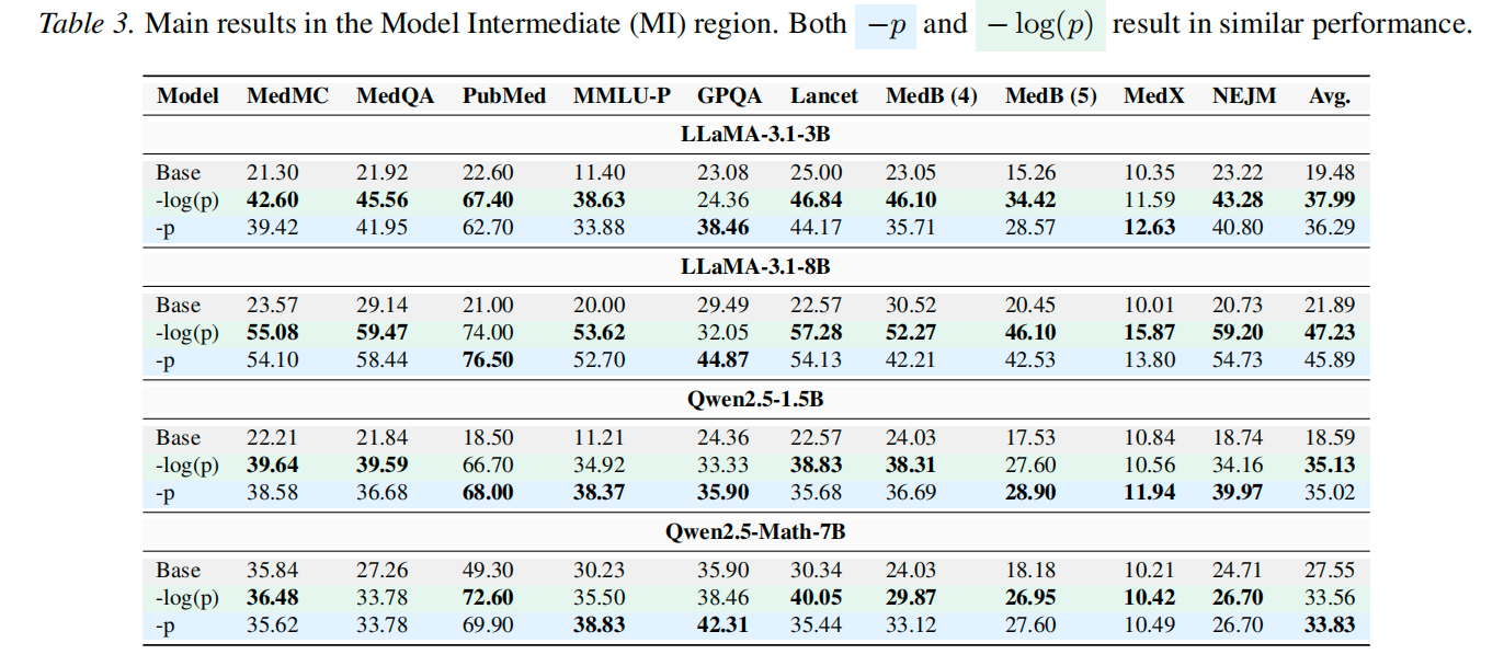
Table 2: Main results in the model-strong end — prior-leaning objectives (−p and thresholded −log p) consistently outperform −log p across models and math datasets

When the model's prior is strong, prior-leaning objectives work better;
When the model's prior is weak, prior-averse objectives work better;
When the model's prior is in between, there is no clear winner.

This means there is no single best SFT loss — the better objective is the one that fits the model.

How to Gauge the Strength of the Model's Prior

Two ways:

Look at the proportion of this data in the model's training corpus;
Look at the model's mean predicted accuracy on the training data.

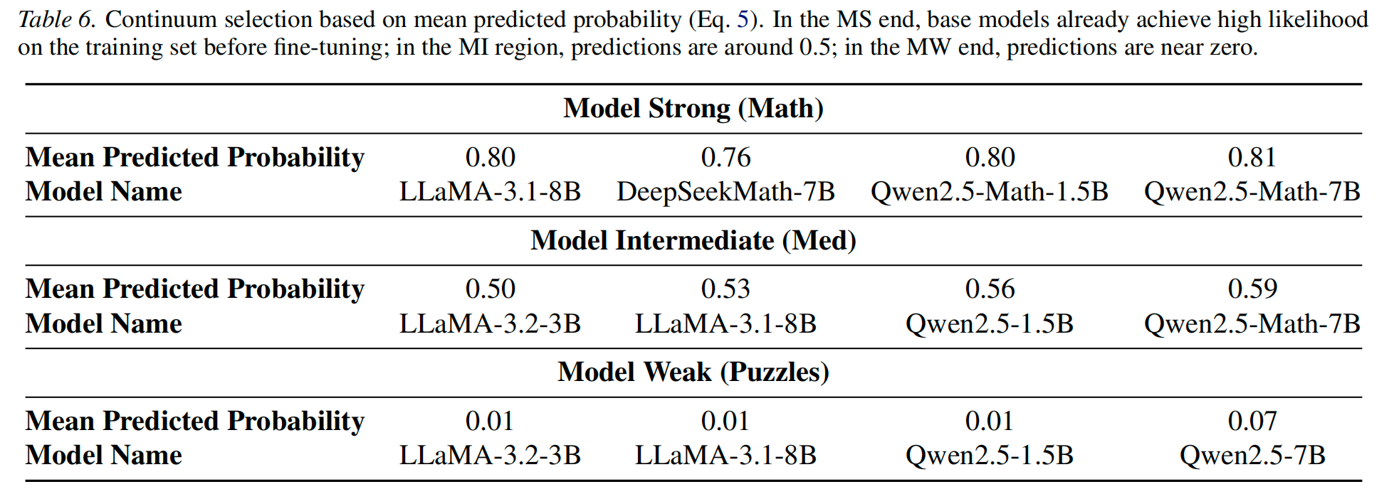
Table 6: Continuum selection based on mean predicted probability — around 0.8 at the model-strong end, around 0.5 in the model-intermediate region, and near zero at the model-weak end

Note that prior strength is jointly determined by both the model and the task: for the same task, it may be a weak prior for model A (favoring prior-averse objectives), but a strong prior for model B (favoring prior-leaning objectives).

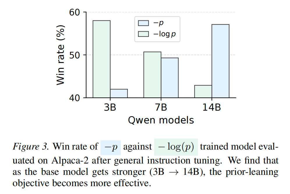
Figure 3: Win rate of −p against −log p evaluated on Alpaca-2 after general instruction tuning — as the base model gets stronger (Qwen 3B → 14B), the prior-leaning objective becomes more effective

Implications for SFT Variants

It is generally believed that online RL is a typical prior-leaning method. Likewise, the SFT variant algorithms I shared before (DFT / ASFT / PSFT) as well as GEM are also prior-leaning.

So these SFT variants are not necessarily superior to NLL — the strength of the model's prior has to be taken into account.

References

[1] Beyond Log Likelihood: Probability-Based Objectives for Supervised Fine-Tuning across the Model Capability Continuum (ICML 2026) — arxiv.org/abs/2510.00526

[2] Official code — github.com/GaotangLi/Beyond-Log-Likelihood

[3] Understanding SFT from an RL Perspective

[4] GEM: Preserving Diversity During SFT